ml-notes
The dangers of L2 (or any other unimodal regression) loss
For better understanding of how the probabilistic modelling principles explained in this post map into actual pytorch code, check out this nice repo made by @shreyansh_26
The problem
What loss function is your first choice when faced with a regression problem? I guess it’s L2. At least that’s what we are taught in intro ML courses. However, as I’ve discovered over my ML engineer career, a lot of ML practitioners don’t fully appreciate the implicit assumptions they make when they use L2, which sometimes leads to gross misinterpretation of the modelling results. I’m guilty of that myself. So in this note I’ll try to summarize what one should be aware of when using L2 or any other unimodal regression loss.
Let’s first remind ourselves what’s the L2 loss. It’s the following function:
\[`L_2(y_{true}, y_{pred}) = (y_{true} - y_{pred})^2.`\]When solving regression problems, the standard approach is to minimize the Monte-Carlo estimate of the expectation of this loss over the data distribution:
\[`\theta^* = \arg \min_{\theta} \frac{1}{|D|} \sum_{(x, y) \in D} \left[f(x; \theta) - y\right]^2.`\]You can then plug $\theta^{*}$ into $f$ to predict $y_{pred} = f(x; \theta^*)$ for any given $x$. This gives us a deterministic rule that connects $x$ and $y.$ But in practice it’s often impossible to predict $y$ from $x$ precisely because we don’t have access to some important information about $y$ and thus can’t put it in $x$, or because the dependency is inherently stochastic1. And the correct way to describe the dependency between $x$ and $y$ is to use the posterior distribution $P(y \mid x)$. So what is this deterministic $y_{pred}$ that we get by solving the regression problem in the standard way, and how does it relate to $P(y \mid x)$?
Turns out, the answer is quite simple: if you assume infinite training data and model capacity, minimization of L2 loss leads to predicting the mean of the posterior $\mathbb{E}_{y \sim P(y \mid x)}[y]$. This can be easily shown:
\[`\mathbb{E}_{y \sim P(y \mid x)} (y_{pred} - y)^2 \to \min`\] \[`\frac{d}{dy_{pred}} \mathbb{E}_{y \sim P(y \mid x)} (y_{pred} - y)^2 = \mathbb{E}_{y \sim P(y \mid x)}\left[2(y_{pred} - y)\right] = 0`\] \[`y_{pred} = \mathbb{E}_{y \sim P(y \mid x)}[y]`\]This fact becomes important when it’s time to make use of $y_{pred}$: interpret its value or plug it into some other function. If you’re fully aware that $y_{pred}$ is an expectation, you should be fine. However, what people often need is not an expectation, but a representative outcome of the process they are trying to model. It can be very subtle: one can unconciously expect good predictions to look similar to the data points in the training set, which are not expectations but samples from the posterior. And the problem is that, depending on the nature of your data, the expectation can be arbitrarily dissimilar to any sample. Let’s consider a few examples.
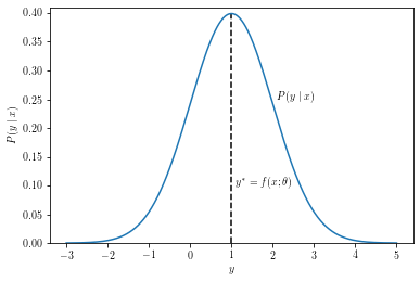
First, the best-case scenario where the L2 regression strives: the posterior is (approximately) symmetrical and unimodal. This, for instance, should happen according to CLT if $y$ is comprised of many independent factors that contribute into it additively, like predicting the height of a person from genetic and environmental data. In this case the expectation of the posterior is representative of the most likely outcome.
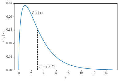
Another possible case is a unimodal posterior with uneven tails. This can happen, for example, if the value you’re trying to model is bounded on one side. For instance, you might be predicting waiting time, which cannot be negative but can be very large. For such problems the expectation of the posterior will correspond to some value that is not entirely unlikely, but can be rather far from the area where most of the outcomes happen.
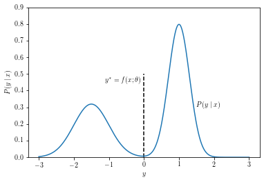
And, finally, we have multimodal distributions. These can arise when the value you are trying to predict depends on some discrete stochastic factor. For example, if you are trying to predict how far a vehicle on the road will travel in 5 sec given its current state, the distance distribution will be multimodal when the vehicle is approaching a yellow traffic light: it will either stop before the stop line or try to pass before the light turns red, but it will likely not maintain its current speed2. When your posterior is multimodal, the expectation might not correspond to any feasible outcome of the process you’re trying to model, and might carry very little information about what is actually going on.
This is not an exhaustive list of modelling setups where using L2 may yield unexpected results. There are, for instance, prediction problems where the output of the model should be a circular quantity such as an angle in $[0, 2\pi]$, and naive L2 application might fail even in a unimodal case. But those are a bit more exotic, and I hope I’ve already convinced you enough that applying L2 loss without understanding the nature of the posterior can yield surprises.
The solution
One way to work around the problem is to think about regression through the prism of probabilistic modelling framework. In this framework, we don’t aim to minimize a loss function, but rather try to maximize the expected log-likelihood of the training data over some parametric distribution family. Turns out, if you try to fit a normal distribution with a feature-dependent mean and a constant variance to your data, this is equivalent to minimizing the L2 loss:
\[`\theta^* = \arg \max_{\theta} \frac{1}{|D|} \sum_{(x, y) \in D} \log \mathcal{N}(y \mid f(x), \sigma^2) =`\] \[`= \arg \max_{\theta} \frac{1}{|D|} \sum_{(x, y) \in D} \left[-\log [\sqrt{2 \pi} \sigma] - \frac{1}{2\sigma^2} (y - f(x))^2 \right] =`\] \[`= \arg \min_{\theta} \frac{1}{|D|} \sum_{(x, y) \in D} \left[y - f(x)\right]^2,`\]where we dropped additive constants and constant scaling factors, which don’t affect the location of the optimum. This view provides another justification for why L2 might not be a good choice: why would you fit a Gaussian to something that doesn’t look like a Gaussian and expect good results?
Thing is, in this framework we have freedom to choose the distribution we are fitting to the data and a recipe for optimization: write down the expected log-likelihood and perform gradient ascent with respect to distribution parameters, this is straightforward to implement in any modern deep learning library. And after we have a well-fitting distribution, we are not restricted to using its mean, we can use any other statistic that is more appropriate for the task (like a mode when you need a representative sample), or even integrate over the whole distribution.
As for the distribution family choice,
- Is the posterior unimodal and sharp? Probably stay with Gaussian.
- Is the posterior unimodal but more heavy-tailed? Laplace might be a better choice3.
- Is the support of the posterior bounded? Maybe you need Beta.
- Is the support bounded from one side? Consider Gamma.
- Are you predicting an angle or other circular quantity? Von-Mises is probably a good choice.
- Is the posterior multimodal? Use a reasonably sized mixture of distributions from the appropriate family.
This, however, mostly applies to scalar outcomes. If you are trying to model a complex object such as an image, it’s likely that no simple parametric distribution family will fit the posterior well. In order to model complex objects you need more expressive families such as autoregressive models, variational autoencoders or diffusion models, but that is out of scope of this note. It should be mentioned, however, that even these advanced methods use the general framework described above: decide on what distribution family you are fitting to the posterior, parametrize it and maximize the log-likelihood of the data (or maybe its approximation or a lower bound if the likelihood is hard to compute exactly).
-
Hidden information and stochasticity are actually the same thing: if you have access to the state of the random generator, everything becomes deterministic. ↩
-
This is a simplified example of an actual modelling problem that is of interest in self-driving industry. ↩
-
This would correspond to minimizing L1 loss in the classical regression setup. ↩